QUESTION A (Convolutional Horses and Humans)
- ImageDataGenerator is a preprocessing tool that can scale and later create generators that hold the data and its corresponding labels. These generators can then be used in the keras library to train the entire generator. One parameter, called the rescale parameter is used to process the image into a certain format, for example normalizing the pixels in an image into the [0,1] range instead of the original [0,255] range. The parameter takes a float that represents the number that will be multiplied into the pixels. In our example, we would set a rescale parameter equal to 1/255 to accomplish our normalization goal of [0,1].
The flow_from_directory method seems to require the base directory (‘/tmp/horse-or-human/’), a target size, a batch size, and a class(ification?) mode. Target size addresses the problem of images with differing dimensions, as this parameter will make sure that all the resulting images that are fed into the initialized generator will be 300x300 pixels. I believe that the class mode is actually short for classification mode. In the video, Moroney talked about how if we had more than one class of data we should use ‘categorical.’ So, make sure to reference the number of classes that this data contains, in this case, there are two classes, horses OR humans, so we use ‘binary.’
The difference between how we define the training and testing generators is the batch size. We used a batch size of 128 for the training generator and a batch size of 32 for the testing generator. The batch size is the number of images that will be taken from the directory to be fed into the neural network. We also use the source directory for the testing images instead of the training images. So instead of using the (‘/tmp/horse-or-human/’) directory, which is for the training images, we use the (‘/tmp/validation-horse-or-human/’) directory, which is for the testing (or validation) images.
- We use three convolution and pooling layers, then flatten the resulting image and pass it through two layers of dense neurons (512 and 1) to get an answer between [0,1] using the sigmoid activation function. I did not modify the number of filters in the convolution layers. As discussed in my previous post July 14th Response, convolutions apply a filter (in this case 3x3) that does not allow the filter to process the pixels on the border of the image, so the image loses 1 pixel in each dimension, causing its dimension to reduce by 2. The max pooling layer halves the dimensions on each side and rounds down.
The sigmoid function for the last dense layer with 1 neuron has a sigmoid activation function. This activation function pushes all outputs toward the [0,1] range. By doing this, we can eliminate the need for using a 2 neuron dense layer and instead use 1. This works only because we have two classes, and we can interpret the output by whether or not it is greater than 0.5. Any output greater than 0.5 is a human, and everything less than or equal to 0.5 is a horse, eliminating the need for a 2 neuron dense layer with only 1 neuron. The rest of the layers are activated by the ‘relu’ (Rectified Linear Unit) function that forces all values toward the positive spectrum. I talk about it in my July 8th Response
QUESTION B (Regression)

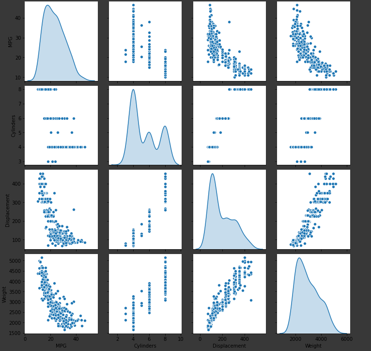
This plt shows the 3x3 relationship between all the variables with the variables correlating to themselves on the y=-x axis. This means that this pairplot function provides visually all the possible combinations between the variables and allows the user to pick up on potential correlations between the variables. For example, there seems to be a exponential relationship between MPG and weight, and a linear relationship between weight and displacement. The function is describing the relationship between each variable including themselves in a plot format.
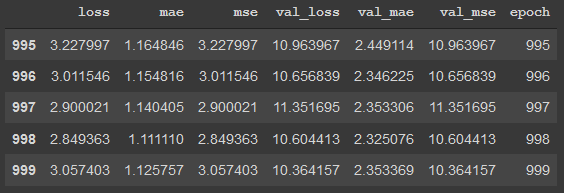
Looking at the chart, I see that the loss is starting to fluctuate around 2.9, the mae and mse seem to be increasing and the val_loss, val_mae, and val_mse are fluctuating. From these observations, it seems that the model is gettin gmore and more overfit as the epochs increase. The training model continues to increase, however the testing model does not.
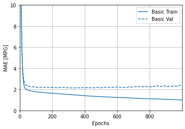
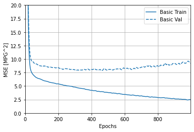
You can see the MSE increasing, and the distance between the training and the testing accuracy diverging at around 100 epochs and increasing all the way to 1000 epochs. The MAE starts diverging at around 25 epochs but stays constant through the 1000 epochs.


QUESTION C (Overfit and Underfit)

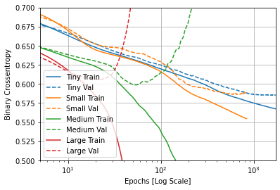
By comparing the 4 different sized models, you can see the differences between the models in terms of how quickly they overfitted to the data. In the case of the largest model, the overfitting happened so fast that you had to switch to a log scale to see whats happening. In this case, comparing the 4 models demonstrates the concept: a larger model has more power to generalize more complex amounts of data, but overfits easily if the model is overqualified to generalize the data set.
